


Better Engineering Through
Multibody Dynamic Simulation
March 2019 | Issue #16
In This Issue:
• New in RecurDyn V9R2: Thermal Load in FFlex, Pre-Stress for Durability and Julia Script for CoLink
• THURSDAY WEBINAR: Optimizing equipment design w/ RecurDyn & EDEM – now with FFlex!
• Particleworks 6.2 Released
• User Tip: Direct definition of an expression to set a parametric value
• User Tip: Create a motion that starts 2 seconds after a certain condition is satisfied
New in RecurDyn V9R2:

Thermal Load in FFlex, Pre-Stress for Durability and Julia Script for CoLink
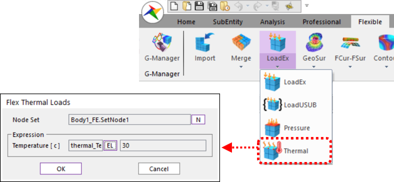
Thermal Load in FFlex
RecurDyn now includes Thermal Loads that can be used in the FFlex module to produce thermal stresses. A Thermal Load consists of temperatures within a pre-created NodeSetAn expression is used to define how the temperature varies with time. The reference temperature is defined in the Material of the corresponding FFlex body. After the analysis is completed, the Thermal Strain can be reviewed and confirmed in the Contour View. The temperature and the thermal strain for each output node can be plotted.
The following Elements are supported:
• Shell3, Shell4
• Solid4, Solid5, Solid6, Solid8
When analyzing RecurDyn models with FFlex bodies, thermal strain and thermal stress can now be included as part of the overall deformation and stress.
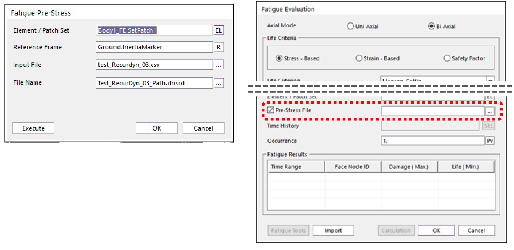
Pre-Stress for Durability
The pre-stress in a flexible body can now be used when performing fatigue analysis using the Durability Toolkit. The newly added ‘Create Fatigue Pre-Stress’ function inputs the Static Stress information for the defined ElementSet or PatchSet into a CSV file format and generates a ‘*.dnsrd’ file (RecurDyn nodal static stress file) containing the Pre-Stress information. When the ‘*.dnsrd’ file is defined as a ‘Pre-Stress File’ in the Fatigue Evaluation dialog, the fatigue analysis results include the effect of the Pre-stress.
For example, if parts are assembled using a press fit, the parts would be Pre-Stressed before the system moves. More accurate fatigue analysis results can be obtained by including the Pre-Stress information.
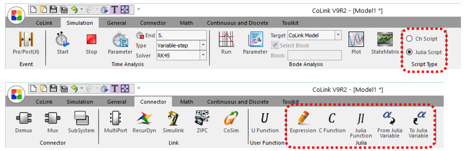
Julia Script in CoLink
CoLink now supports Julia Script and the functions related to Julia Script have been added to user-defined blocks. The functions related to Julia Script can be found in the Connector tab of CoLink after selecting Julia Script in the Script Type in the Simulation tab of CoLink.
Julia Script will feel familiar to many users because it is similar to MATLAB Commands and Scripts. The advantages of using Julia Script include:
• Does not require variable declarations
• Can be linked with the C library
• Matrix operations are quick and easy
• Various libraries and related materials can be easily obtained and utilized
Various blocks, including user-developed algorithms, can be created using the related functions of Julia Script. Customized CoLink models can be created by linking with existing blocks and used for CoLink analysis. For example, Julia Script can be used to create a control block containing the user’s know-how, which is optimized for the specific simulation environment and requirements, and it can be used for control simulation using RecurDyn.
Webinar:
Optimizing Equipment Design with RecurDyn & EDEM – now with FFlex
The latest versions of EDEM and RecurDyn introduced the ability for EDEM bulk materials to interact with the non-linear FFlex body in RecurDyn. This enable the prediction of deformation and stress within individual parts as a function of contacts with bulk materials. The result is greater realism and insight into real-world systems. This webinar will show examples of this new flexible geometry modeling capability.

Background: Multi-body and systems dynamics simulation is critical in the design of heavy equipment and off-road vehicles. When using tools such as RecurDyn, by FunctionBay, it is essential that there are accurate representations of ALL the loads acting on a piece of equipment. This includes forces generated by the bulk materials that machinery and vehicles interact with (such as soil, rocks, gravel, mined ores etc.). Combining RecurDyn and EDEM in a co-simulation environment enables engineers to have accurate, dynamic bulk material load inputs in their MBD simulations as standard. This means increased realism in equipment motions and also a complete understanding of how bulk material loads are transferred throughout their mechanical system.
Date: Thursday 14 March, 2019 [2 times offered]
Duration: 40 minutes + time for questions
Presenter: Sophie Broad, Senior EDEM Engineer
Topics covered:
• Challenges of heavy equipment design
• Introducing EDEM bulk material simulation software
• Overview of EDEM-RecurDyn coupling:
• Applications and benefits
• Flexible geometry modeling
• Examples: excavator, tracked vehicle and more
• Workflow
• Live Q&A with our engineer
* All registrants will receive a recording afterwards so you are encouraged to register even if you cannot attend on the day.
RecurDyn News & Tips
User Tip:
Direct definition of an expression to set a parametric value
A Parametric Value (PV) is an essential entity for use in parametric modeling. Intelligence can be added to a model when a PV can be defined as a function of another parametric variable. In this case the user can change a single PV and changes can spread to other PVs. This intelligence requires that the PV is defined as an expression, which sometimes is a cumbersome process.
The Value of a PV can be directly input as an expression, as shown below:
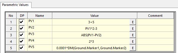
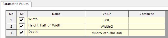
Please consider an example model where 2 PVs are defined as a function of an independent PV to define the geometry of a box, as shown below.
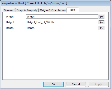
The PVs are used in the box property dialog, as shown below.
First, the width of a box is defined as an independent variable which starts with the value of 800. Second, the height of the box is defined to be one half of the width. Third, the depth of the box is defined as being the maximum of the width minus 300 or 200.
For example, if the Width PV is 800, then the Height_Half_of_Width is 400 and the Depth PV is 500.
Likewise, if the Depth PV is 400, then the Height_Half_of_Width is 200 and the Depth PV is 200.
Using this technique, you can easily and quickly create a parametric model with geometry that morphs in multiple ways when a single parametric value is changed.
User Tip:
How can you easily apply supplier data to your RecurDyn model when the supplier data is provided in different units?
Option 1: A motion that starts 2 seconds after an event can be easily implemented using the IF function. For example, if you use a function
IF(time-2 : 0, 0, (time-2)*100)
as a motion of the translational joint, the motion is 0 for the first 2 seconds and the motion is (time-2)*100 starting at 2 seconds. For example, the motion is 0 at 2 seconds, 100 at 3 seconds, and 200 at 4 seconds.
Option 2: A motion that takes 2 seconds before starting moving after a certain condition is met can be easily implemented using the Signal Chart of CoLink.But what if you don’t use CoLink?
Option 3: If you don’t use CoLink, you can use a Laser Sensor. It is triggered when a specified body (geometry) is within a certain sensor range. An example definition of the Laser Sensor is shown below.

An expression function, SENSORONTIME(…) returns the time when the sensor is triggered. We can utilize this function. Please read the below explanation first, then review the model by clicking here.
If a specified condition is met, move a dummy body to a location which is within the sensor range.
Then SENSORONTIME will return the time when the condition is met.
Then use SENSORTIME(…) as shown in the function below.
SENSOR (LaserSensor1) *
(time > (2 + SENSORONTIME(LaserSensor1))) *
(time – (2 + SENSORONTIME(LaserSensor1)) ) * 100
The explanation of this expression is:
SENSOR(LaserSensor1): returns 1 if the sensor is triggered, or returns 0.
(time > (2+SENSORONTIME(LaserSensor1)): returns 1 after 2 seconds of triggered time, or returns 0.
(time – (2+SENSORONTIME(LaserSensor1)) )*100: This is the expression you desire to apply as a motion.
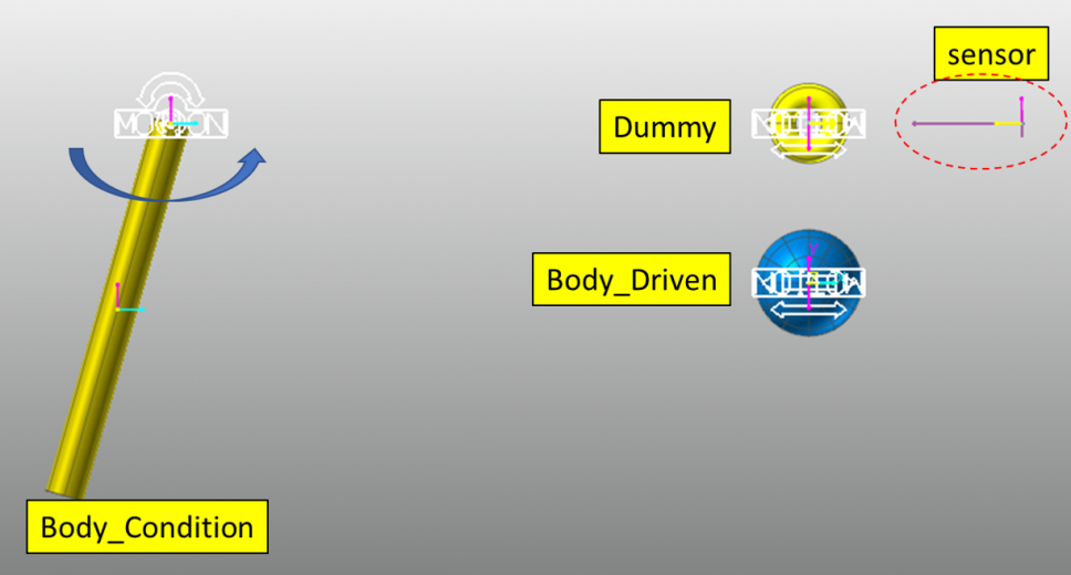
Description of the linked model.
The target is to implement an expression to move Body_Driven to the right side 2 seconds after Body_Condition rotates more then 1 radian.
Steps to creating the model:
- Create a Dummy body. When Body_Condition rotates 1 rad, move it to the location where it is within the sensor range of ‘LaserSensor1’
- Since displacement and angle functions such as DX(1, 2) cannot be used to define a Motion, you need to use a variable equation (VE1) instead.
- Create an expression with the SENSORONTIME(LaserSensor1) causing the motion to move Body_Driven
- SENSORONTIME(LaserSensor1) returns the time when the sensor is triggered (when the Body_Condition rotates 1 rad)
Want to learn more about how MotionPort can help you with your projects? Contact us today to schedule a free web meeting to learn how RecurDyn, Particleworks, and MBD for ANSYS are helping our clients and how they can help you.
MotionPort LLC | St. George, UT | www.motionport.com
Click here to unsubscribe