


Modeling Contacts
Many mechanical systems include contacts and the simulation of contacts can use up a lot of calculation time. It is important to be able to calculate the contacts quickly while maintaining sufficient accuracy. RecurDyn provides a broad library of 3D and 2D contacts to choose from when creating a model, as shown in the figure.
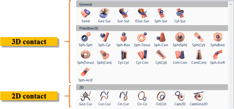
3D Contact
A 3D contact defines the contact between two three-dimensional shapes. The solid contact (Solid) and geo surface (Geo Sur) contacts are widely used because they can be quickly defined between bodies with general geometry. We will discuss how to use these below as well as the Primitive3D contacts.
You can download a RecurDyn model using the link below to reference as you continue reading this guide.
3D Contact Example Model Download
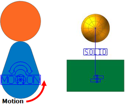
An example use of a Solid Contact, which is a 3D Contact
2D Contact
A 2D contact is defined between two curves, although one or both of the curves can be a special case for a curve, a circle. Although RecurDyn models generally consider 3D assemblies, sometimes the mechanism in the assembly has 2D motion, as constrained by several joints. In this case contact between two bodies can be described using a 2D contact, which solves more quickly. A 3D contact may be preferred if there is interest is observing contact pressures.
The most widely used 2D contact is a geo curve (Geo Cur).
You can download a RecurDyn model using the link below to reference as you continue reading this guide.
A Model Expressed with a Curve-to-Curve Contact Object, which is a 2D Contact Object
Tip: You may use the curve constraints, PTCV and CVCV, in order to reduce the simulation time as compared to using 2D contacts. The disadvantage would be that the bodies would no longer have the ability to “lift off.” Please refer to the following FAQ “How can I reduce the time required to analyze a model that includes contacts (PTCV, CVCV)?” for more information about using the PTCV and CVCV contraints.
Using Contacts
Note: Contact objects can be used in a variety of ways depending on the entities in the model, such as its geometries and parameters. Therefore, the following information should be used as a basic guide to working with contacts. The contacts in a specific model may behave differently than described in this guide.
Solid Contact
Solid contacts are fast and accurate when contact occurs between two general convex surfaces or between a flat surface and a convex surface (examples shown in the figure to the right).
The figure below shows a model in which several small spheres exist inside a larger sphere.
In this example, contact occurs between the convex surfaces of the small spheres and the concave surface of the larger sphere.
However, as the contact occurs only in small portions of the spheres rather than large areas, solid contact objects may still be applied successfully because the concave contact surface of the large sphere is sufficiently flat to properly interact with the convex surfaces of the small spheres.
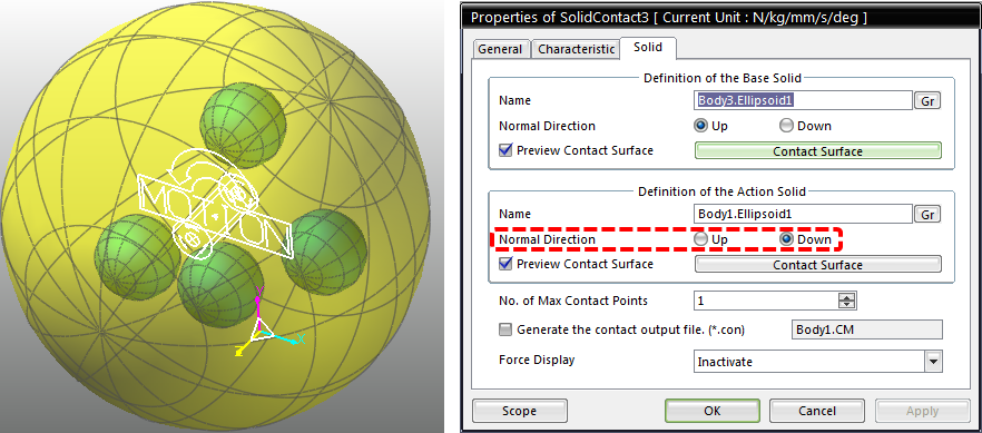
When you define a contact inside a shape, as shown above, you may need to adjust the Normal Direction in the Solid tab of the Properties dialog box (as highlighted).
Geo Surface Contact
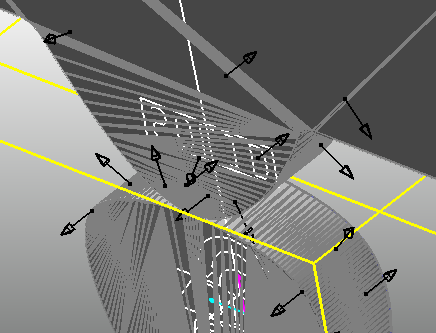
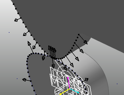
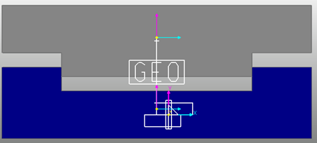
Geo surface contact objects can be applied to almost any form of contact. If the contact occurs between two convex surfaces, however, a solid contact object will produce faster analysis results than a geo surface contact object. As we stated before, a geo surface contact object works better than a solid contact object when contact occurs between flat surfaces or contact occurs over a large area between a convex surface and a concave surface. The figure illustrates one such case, where the convex surface of the upper body fits tightly within the concave surface of the lower body.
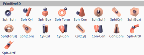
Primitive 3D Contact Objects
The two contacts described above are good choices for bodies with general surfaces. In some cases a bodies may include a contact surface that can represented with an analytical shape, such as a sphere, box, or cylinder. An example of this would be the contact between a pin and a hole. This could be efficiently modeled with a cylinder-in-cylinder contact. The Primitive3D contacts, as shown in the figure, can be used to model these analytical contacts quickly and accurately. Please note the dash symbol (“-“) in the contact names can be replaced with the word “to.” The left parentheses can be replaced with the word “in.” Therefore the contact name Sph-Sph is a short version of “Sphere-to-Sphere” and Sph(Sph) is a short version of “Sphere-in-Sphere.”
The reason that the primitive contacts are fast, smooth, and accurate is that the contact surfaces can be expressed mathematically, so the RecurDyn solver needs to consider only a few equations in order to determine the accurate contact point and calculate the contact force.
The primitive 3D shapes may be created manually in RecurDyn or they will be created for you if you have the right option turned on when you import a CAD file. The option is “Convert Primitive Geometries when importing CAD Files” and it is found in the CAD dialog box that is shown when you click on the CAD option under the pull-down menu that includes the Display setting, within the Setting group of the ribbon under the Home tab. It can be worthwhile to invest some time to arrange to have primitive geometry in your RecurDyn model so that you can take advantage of Primitive 3D contacts.
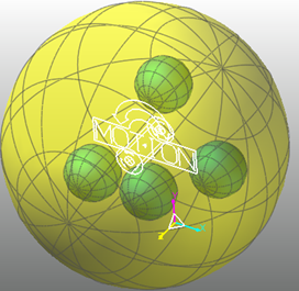
For example, with the model described in the “Solid Contact” section, you could use a sphere-to-sphere contacts and sphere-in-sphere contacts to run simulations that are at least ten times faster than when solid contacts are used.
For piston models, you could use a cylinder-in-cylinder contact object. For bearing models, you could use a sphere-in-torus contact object.
Although general contact objects can be used regardless of the shape of the object and are needed to represent complex geometry, you may want to use primitive 3D contacts when possible to obtain fast and accurate analysis results.
Basics of the Contact Algorithm
Given the potential for contact analysis to occupy most of the calculations and to affect the simulation results, it is very important to understand the basics of the contact algorithm and contact parameters.
RecurDyn contact is based on the penalty method, which is of the most common contact algorithms. There are many possible ways to implement the penalty method, and the performance and accuracy depend on the implementation. Fundamentally, the key characteristic of the penalty method is that it uses the interference between the bodies in contact to calculate the contact force.
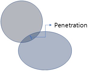
Let’s consider the figure to the right. The bodies are in contact with each other. In reality, the material of the two bodies are not overlapped, but the bodies deform in response to the contact force.
The penalty method uses the concept of the overlapped material (‘penetration’) and the concept of ‘penetration depth’ to define the equivalent of a deformed spring to calculate the contact force. This is the basic concept of the penalty method.
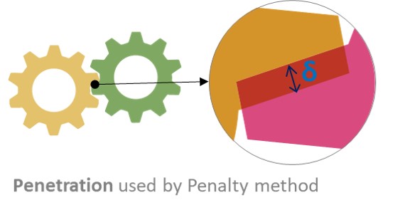
The Penalty Method calculates the contact force as if there is a spring between the ‘overlapped area’ and the spring is compressed by the penetration.
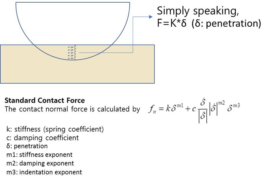
In other words, if the penetration is δ, the contact force f is calculated by f = kδ. (K is one of the contact parameters, Stiffness Coefficient.)
The equation for determining the contact force is shown in the figure to the right.
There are other factors that are considered as well, as shown in the figure. The damping portion of the contact force is a function of the relative velocity between bodies and always opposes the relative motion. The damping force is also a function of the penetration.
There are three exponents that can be used to tune the contact force in order to achieve the most realistic behavior. Many RecurDyn beginners use contacts without knowing the details of the contact force calculation. But you will be able to use RecurDyn contacts and set the contact parameters successfully if you understand the contact force calculation. You can also contact MotionPort for advice on selecting contacts and setting the contact parameters.
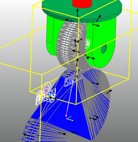
For bodies with complex geometry, the contact surface is divided into small, flat facets that are used to identify when interferences occur and to find the location contact point for that simulation time.
Consequently, a small deviation occurs between the actual shape of the geometry and the shape that is defined by the facets. RecurDyn will automatically place more (smaller) facets in area of high curvature. You can also control the size of the facets by adjusting properties of each contact surface.
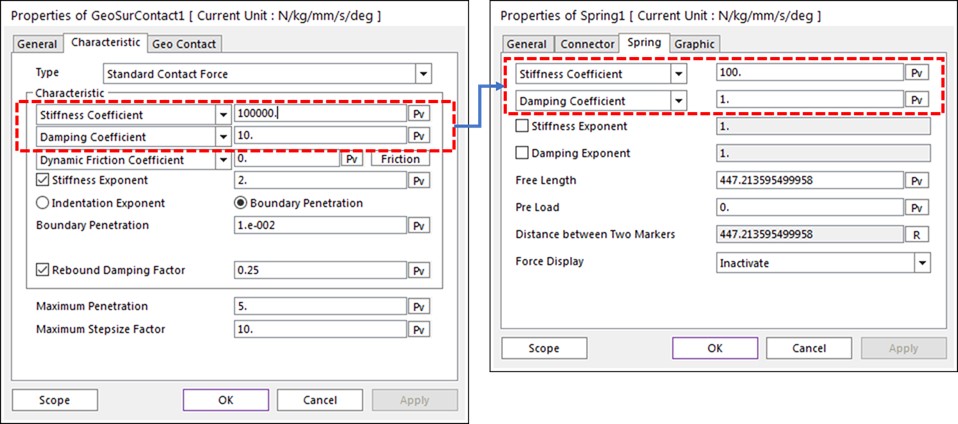
Each type of contact has a Characteristic tab in the associated Properties dialog box.
The Stiffness and Damping Coefficients for the contact perform the same functions as the Stiffness and Damping Coefficients in the Spring Force dialog box, as shown in the figure below.
The explanation in this document is to help your understanding of the Penalty method. The MotionPort website has a collection of technical papers about contact modeling at https://motionport.com/resources/technical-papers/contact-modeling. Please refer to these papers for the theoretical description of the Penalty method as well as other contact techniques.)
Example Contact Calculation
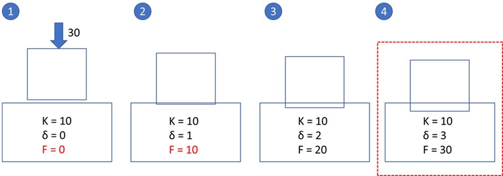
In the example image below, we consider a sequence of four cases where the penetration increases until the external force and the contact force (f = kδ) reach equilibrium. Note that units are not specified for simplicity.
Case #1 – The weight of the upper box applies a force of 30, but there is no contact force because there is no penetration (δ=0). Consequently, the upper box moves downward.
Case #2 – There is penetration, δ=1, so a contact force of 10 occurs, but since the weight of the upper box (30) > 10, the box continues to move downward.
Case #3 – Since 30 > 20, so the box continues to move downward.
Case #4 – Finally at a penetration of 3 the force equilibrium is achieved (30 = 30).
Note that the example values of δ are quite large in this example. This was done to help you visualize the contact calculation. However, with real models the value of δ is typically quite small.
Since the contact force f = kδ, if you set K (stiffness coefficient) too small, δ must be very big to achieve the force equilibrium. In fact, penetration (δ) is an artificial value so very small δ is reasonable. Therefore, it is good to use a big enough value for K. For example, the default K of the RecurDyn Geo Surface Contact and Solid Contact is 100,000 N/mm.)
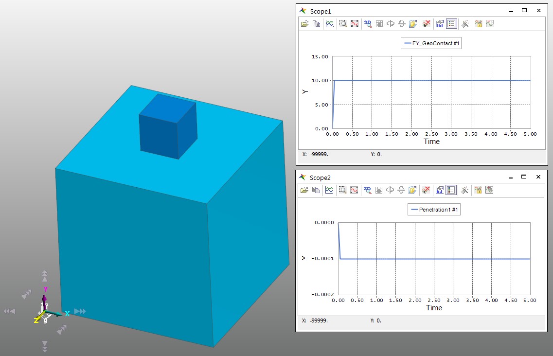
In the below example, a box whose mass is 1Kg is put on a big box. In this case, the contact force is calculated to be approximately 10N (assuming that the gravitational acceleration is approximately 10m/s^2) and the penetration is 0.0001 mm when K = 100,000 N/mm.
If K is too big, since f = kδ, a small change of the penetration (δ) affects the magnitude of the contact force drastically. If the contact force changes a lot, it can make the RecurDyn solver unstable. High stiffness coefficients can result in high frequency vibrations in the system. Therefore, it is very important to use the appropriate K for each situation. In summary, if K is too small excessive penetration occurs and the result becomes inaccurate. But if K is too big, the large force variation affects the solver stability. When tuning the stiffness coefficient it is best to adjust the value higher or lower by no more that a faction of ten with each adjustment.
Example Contact Cases
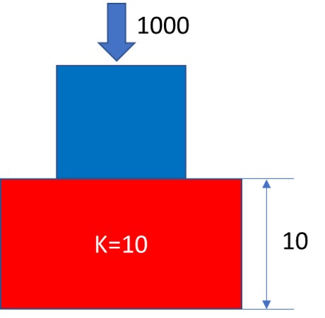
Case #1:
In this figure, let’s assume that the blue (small) box is very heavy. The mass is 100 kg, and the downward force is approximately 1000 N)
– If K = 10N/mm, δ must be 100 mm to achieve a force equilibrium (when the contact force = 1000N).
– If the height of the red box is 10mm, δ cannot be 100mm. So, in this model the blue box will fall down through the red box because the force equilibrium is not achieved.
Solution #1:
Sometimes there is excessive penetration between the two bodies. Please remember that this is usually caused by too big external force or too small K. If you want to reduce the penetration, increase K. If you can predict the magnitude of the contact force, you can estimate the minimum K for the simulation (the appropriate K). For example, if you set K = 100,000 N/mm, then the force equilibrium can be achieved when δ=0.01mm.)
Case #2:
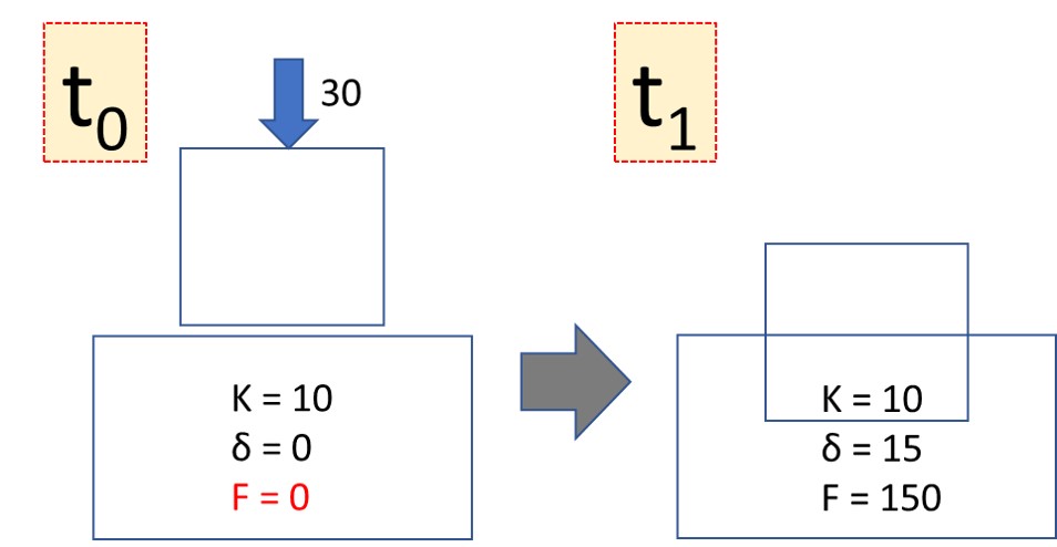
Numerical analysis uses the discrete time steps for the calculation. Therefore, when the time step is big (as in the figure) and the relative velocity between bodies is significant, contact may not occur between 2 bodies at the starting time step and then the 2 bodies can overlap excessively at the next time step. In the below model, at the first time step (t0), δ = 0, so only gravity is applied to the upper box and it moves downward.
If δ becomes 15 at t1, the upward force (contact force) becomes 150 and the downward force (gravity) is still 30. The net force becomes an upward force of 120 (150 – 30). As a result, the upper box can suddenly bounce upward because of the abrupt upward force that is applied to the upper box.
Solution #2:
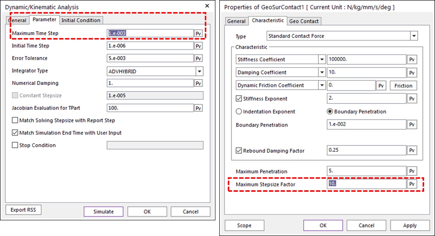
To avoid this kind of trouble, you should use the sufficiently small time step size to prevent the sudden large penetration. You can use the RecurDyn solver parameter, Maximum Time Step to ensure a small time step. The experienced users can use Maximum Stepsize Factor in the Contact parameter dialog instead. This parameter uses a smaller time step when the contact between 2 bodies is active.
For example, consider a Maximum Stepsize Factor = 10 in the below (right-side) dialog. When 2 bodies are about to be contacted (as they approach each other), RecurDyn solver reduces the time step by a factor of 10 to prevent the excessive penetration by the sudden collision.
Case #3:
This case is similar to Case #1, where it is possible that the upper body just falls through the lower body instead of bouncing off.
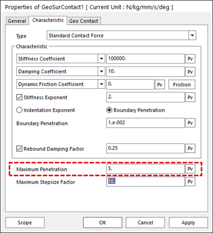
This kind of result may be caused by the Maximum Penetration in the Contact parameter dialog. This parameter means that if the real penetration is bigger than this ‘Maximum Penetration’, the contact force is not calculated. This is needed to prevent false contacts when one body passed around and behind the other body.
In this case, if the Maximum Penetration is set to 5, since δ = 15 at t1, the contact force becomes 0 because 15 > 5. As a result, only the downward force (30) is applied to the upper box, and the upper box continues to fall down.
Solution #3:
The solution is also similar to the Solution #2, that the time step size needs to be reduced to prevent the excessive penetration. Technically, increasing the maximum penetration can prevent this kind of problem, but it is recommended to reduce the time step size in most cases because the smaller penetration produces the better result.
Again, please remember that the MotionPort website has a collection of technical papers about contact modeling at https://motionport.com/resources/technical-papers/contact-modeling.
 In earlier versions of